
2.1 Linear Phase
2.1.1 What is the association between FIR filters and “linear-phase?”
Most FIRs are linear-phase filters; when a linear-phase filter is desired, a FIR is usually used.
2.1.2 What is a linear phase filter?
“Linear Phase” refers to the condition where the phase response of the filter is a linear (straight-line) function of frequency (excluding phase wraps at +/- 180 degrees). This results in the delay through the filter being the same at all frequencies. Therefore, the filter does not cause “phase distortion” or “delay distortion”. The lack of phase/delay distortion can be a critical advantage of FIR filters over IIR and analog filters in certain systems, for example, in digital data modems.
2.1.3 What is the condition for linear phase?
FIR filters are usually designed to be linear-phase (but they don’t have to be.) A FIR filter is linear-phase if (and only if) its coefficients are symmetrical around the center coefficient, that is, the first coefficient is the same as the last; the second is the same as the next-to-last, etc. (A linear-phase FIR filter having an odd number of coefficients will have a single coefficient in the center which has no mate.)
2.1.4 What is the delay of a linear-phase FIR?
The formula is simple: given a FIR filter which has N taps, the delay is: (N – 1) / (2 * Fs), where Fs is the sampling frequency. So, for example, a 21 tap linear-phase FIR filter operating at a 1 kHz rate has delay: (21 – 1) / (2 * 1 kHz)=10 milliseconds.
2.1.4 What is the alternative to linear phase?
Non-linear phase, of course. 😉 Actually, the most popular alternative is “minimum phase”. Minimum-phase filters (which might better be called “minimum delay” filters) have less delay than linear-phase filters with the same amplitude response, at the cost of a non-linear phase characteristic, a.k.a. “phase distortion”.
A lowpass FIR filter has its largest-magnitude coefficients in the center of the impulse response. In comparison, the largest-magnitude coefficients of a minimum-phase filter are nearer to the beginning. (See dspGuru’s tutorial How To Design Minimum-Phase FIR Filters for more details.)
2.2 Frequency Response
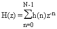
2.2.1 What is the Z transform of a FIR filter?
For an N-tap FIR filter with coefficients h(k), whose output is described by:
y(n)=h(0)x(n) + h(1)x(n-1) + h(2)x(n-2) + … h(N-1)x(n-N-1),
the filter’s Z transform is:
H(z)=h(0)z-0 + h(1)z-1 + h(2)z-2 + … h(N-1)z-(N-1) , or
2.2.2 What is the frequency response formula for a FIR filter?
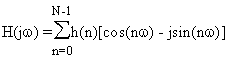
The variable z in H(z) is a continuous complex variable, and we can describe it as: z=r·ejw, where r is a magnitude and w is the angle of z. If we let r=1, then H(z) around the unit circle becomes the filter’s frequency response H(jw). This means that substituting ejw for z in H(z) gives us an expression for the filter’s frequency response H(w), which is:
H(jw)=h(0)e-j0w + h(1)e-j1w + h(2)e-j2w + … h(N-1)e-j(N-1)w , or
Using Euler’s identity, e-ja=cos(a) – jsin(a), we can write H(w) in rectangular form as:
H(jw)=h(0)[cos(0w) – jsin(0w)] + h(1)[cos(1w) – jsin(1w)] + … h(N-1)[cos((N-1)w) – jsin((N-1)w)] , or
2.2.3 Can I calculate the frequency response of a FIR using the Discrete Fourier Transform (DFT)?
Yes. For an N-tap FIR, you can get N evenly-spaced points of the frequency response by doing a DFT on the filter coefficients. However, to get the frequency response of the filter at any arbitrary frequency (that is, at frequencies between the DFT outputs), you will need to use the formula above.
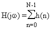
2.2.4 What is the DC gain of a FIR filter?
Consider a DC (zero Hz) input signal consisting of samples which each have value 1.0. After the FIR’s delay line had filled with the 1.0 samples, the output would be the sum of the coefficients. Therefore, the gain of a FIR filter at DC is simply the sum of the coefficients.
This intuitive result can be checked against the formula above. If we set w to zero, the cosine term is always 1, and the sine term is always zero, so the frequency response becomes:
2.2.5 How do I scale the gain of a FIR filter?
Simply multiply all coefficients by the scale factor.
2.3 Numeric Properties
2.3.1 Are FIR filters inherently stable?
Yes. Since they have no feedback elements, any bounded input results in a bounded output.
2.3.2 What makes the numerical properties of FIR filters “good”?
Again, the key is the lack of feedback. The numeric errors that occur when implementing FIR filters in computer arithmetic occur separately with each calculation; the FIR doesn’t “remember” its past numeric errors. In contrast, the feedback aspect of IIR filters can cause numeric errors to compound with each calculation, as numeric errors are fed back.
The practical impact of this is that FIRs can generally be implemented using fewer bits of precision than IIRs. For example, FIRs can usually be implemented with 16 bits, but IIRs generally require 32 bits, or even more.
2.4 Why are FIR filters generally preferred over IIR filters in multirate (decimating and interpolating) systems?
Because only a fraction of the calculations that would be required to implement a decimating or interpolating FIR in a literal way actually needs to be done.
Since FIR filters do not use feedback, only those outputs which are actually going to be used have to be calculated. Therefore, in the case of decimating FIRs (in which only 1 of N outputs will be used), the other N-1 outputs don’t have to be calculated. Similarly, for interpolating filters (in which zeroes are inserted between the input samples to raise the sampling rate) you don’t actually have to multiply the inserted zeroes with their corresponding FIR coefficients and sum the result; you just omit the multiplication-additions that are associated with the zeroes (because they don’t change the result anyway.)
In contrast, since IIR filters use feedback, every input must be used, and every input must be calculated because all inputs and outputs contribute to the feedback in the filter.
2.5 What special types of FIR filters are there?
Aside from “regular” and “extra crispy” there are:
- Boxcar – Boxcar FIR filters are simply filters in which each coefficient is 1.0. Therefore, for an N-tap boxcar, the output is just the sum of the past N samples. Because boxcar FIRs can be implemented using only adders, they are of interest primarily in hardware implementations, where multipliers are expensive to implement.
- Hilbert Transformer – Hilbert Transformers shift the phase of a signal by 90 degrees. They are used primarily for creating the imaginary part of a complex signal, given its real part.
- Differentiator – Differentiators have an amplitude response which is a linear function of frequency. They are not very popular nowadays, but are sometimes used for FM demodulators.
- Lth-Band – Also called “Nyquist” filters, these filters are a special class of filters used primarily in multirate applications. Their key selling point is that one of every L coefficients is zero–a fact which can be exploited to reduce the number of multiply-accumulate operations required to implement the filter. (The famous “half-band” filter is actually an Lth-band filter, with L=2.)
- Raised-Cosine – This is a special kind of filter that is sometimes used for digital data applications. (The frequency response in the passband is a cosine shape which has been “raised” by a constant.) See dspGuru’s Raised-Cosine FAQ for more information.
- Lots of others.