
by Rick Lyons
Performing interpolation on a sequence of time-domain samples is an important (often used) process in DSP, and there are many descriptions of time-domain interpolation (a kind of curve fitting) in the literature and on the Internet. However, there’s a lesser-known scheme used for interpolation that employs the inverse discrete Fourier transform (IDFT). This little tutorial attempts to describe that technique.
One of the fundamental principles of discrete signals is that “zero padding” in one domain results in an increased sampling rate in the other domain. For example, the most common form of zero padding is to append a string of zero-valued samples to the end of some time-domain sequence. Looking at a simple example of this notion, Figure 1(a) shows a Hanning window sequence w(n) defined by 32 time samples. If we take a 32-point DFT of w(n), and just look at the magnitudes, we get the WdB(m) spectral magnitude plot shown in Figure 1(b).

Figure 1
If, on the other hand, we zero pad (append) 96 zero-valued samples to the end of w(n), we’ll have the 128-sample w’(n) sequence shown in Figure 1(c). The spectral magnitude plot of a 128-point DFT of w’(n) is shown in Figure 1(d), where we can see the more detailed structure of the Fourier transform of a Hanning window. So, in this case, we can say “zero padding in the time domain results in an increased sampling rate in the frequency domain”. Here the zero padding increased our frequency-domain sampling (resolution) by a factor of four (128/32).
For each sample in Figure 1(b), we have four samples in Figure 1(d).
Many folk call this process “spectral interpolation”.
OK, that’s time-domain zero padding. No big deal, you’ve probably seen this before. Now let’s see what frequency-domain zero padding (FDZP) will do for us by way of an example. Think of an 8-sample real discrete sequence comprising the sum of a 1 kHz and a 2 kHz sinusoids defined as:
x(n)=sin(2·pi·1000·nts) + 0.5sin(2·pi·2000·nts + 3·pi/4),
where ts is the sample period (1/fs), and the fs sample rate is 8000 samples/second. Our eight x(n) samples are shown as the black dots in Figure 2.
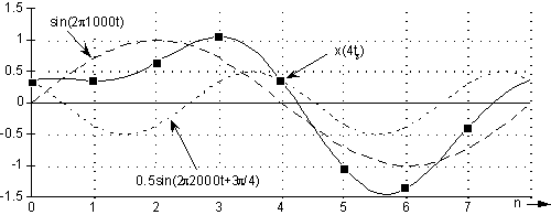
Figure 2
We’ll call x(n)’s 8-point DFT the frequency-domain sequence X(m), the real and imaginary parts of which are shown in Figure 3(a) and 3(b). OK, here’s where the zero padding comes in. If we insert 8 zero-valued complex samples in the middle of X(m), we’ll have a new complex spectrum whose real and imaginary parts are shown in Figure 3(c) and 3(d). Realize, now, that a complex zero is merely 0 + j0.
That “middle of X(m)” phrase means just prior to half the sample rate, or 4 kHz in this example. Because of the way the X(m)’s sample index numbering is mapped to the frequency-domain axis, we can think of this fs/2 = 4 kHz point as the highest positive frequency in the spectrum. Thus we insert the zeros after the first N/2 spectral samples, where N is the length of X(m), in order to maintain spectral symmetry. (We’re assuming that the 4 kHz, X(N/2), spectral component is zero, or at least negligibly small, in magnitude.)
OK, let’s call this new 16-sample discrete spectrum X’(m).
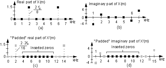
Figure 3
Now, here’s the slick part. If we take a 16-point inverse DFT of X’(m), we’ll get the interpolated time sequence shown in Figure 4. Check it out! In between each of the original x(n) samples (shaded dots), we’ve calculated the intermediate time samples (the black dots). All 16 dots in Figure 4 represent the new interpolated 16-sample x’(n) sequence. In this case, we can say “zero padding in the frequency domain results in an increased sampling rate in the time domain”.
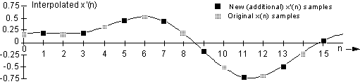
Figure 4
A few things to keep in mind about this FDZP technique:
1.) Notice the agreeable property that the FDZP’s interpolated time samples match the original time samples. (The shaded dots in Figure 4.)
2.) We must not append zeros to the end of the X(m) sequence, as occurs in time-domain zero padding. The complex zero padding must take place exactly in the middle of the original X(m) sequence, with the middle frequency sample being fs/2.
3.) The new time sequence x’(n), the inverse DFT of X’(m), is complex. However, if we stuffed the zeros properly X’(m) will symmetrical and x’(n)’s imaginary parts should all be zero (other than very small computational errors). Thus Figure 4 is a plot of the real parts of x’(n).
4.) Notice how the amplitudes of the new x’(n) time sequence were reduced by a factor of two in our example. (This amplitude reduction can, of course, be avoided by doubling either the X’(m) or the x’(n) amplitudes.)
5.) In Figure 4 we interpolated by a factor of two. Had we stuffed, say, 24 zeros into the X(m) sequence, we could perform interpolation by a factor of four using the inverse fast Fourier transform (IFFT). The point here is that the number of stuffed zeros must result in an X’(m) sequence whose length is an integer power of two if you want to use the efficient radix-2 inverse FFT algorithm. If your new X’(m) sequence’s length is not an integer power of two, you’ll have to use the inverse discrete Fourier (IDFT) transform to calculate your interpolated time-domain samples.
Although I haven’t gone through a mathematical analysis of this scheme, the fact that it’s called “exact interpolation” in the DSP literature is reasonable for periodic time-domain sequences. Think of the standard technique used to perform time-domain interpolation using a low-pass FIR filter. In that method, zero-valued samples are inserted between each of the original time samples, and then the new (lengthened) sequence is applied to an FIR filter to attenuate the spectral images caused by the inserted zeros. The accuracy of that FIR filter interpolation technique depends on the quality of the filter. The greater the low-pass FIR stopband attenuation, the greater the image rejection, and the more accurate the time-domain interpolation. In this FDZP technique, for periodic time signals, image rejection is ideal in the sense that the spectral images all have zero amplitudes.
If our original time-domain sequence is not periodic, then the FDZP scheme exhibits the Gibbs’ phenomenon in that there will be errors at the beginning and end of the interpolated time samples. When we try to approximate discontinuities in the time-domain, with a finite number of values in the frequency-domain, ripples occur just before and after the approximated (interpolated) discontinuity in the time-domain. Of course, if your original time sequence is very large, perhaps you can discard some of the initial and final erroneous interpolated time samples. From a practical standpoint, it’s a good idea to model this FDZP technique to see if it meets the requirements of your application.
One last thought here. For those readers with Law Degrees, don’t try to cheat and use this FDZP technique to compensate for failing to meet the Nyquist sampling criterion when your x(n) time samples were originally obtained. This interpolation technique won’t help because if you violated Nyquist to get x(n), your X(m) DFT samples will be invalid due to aliasing errors. This FDZP scheme only works if Nyquist was satisfied by the original x(n).
About the Author:
Rick Lyons is the author of the best-selling DSP book Understanding Digital Signal Processing [Lyo97], and also teaches the short course Digital Signal Processing Made Simple For Engineers.
© 1999 Richard G. Lyons ![]() Used with permission.
Used with permission.